In machine learning online course taking in, there's something many refer to as the "No Free Lunch" hypothesis. More or less, it expresses that nobody calculation works best for each issue, and it's particularly important for managed learning (i.e. prescient demonstrating).
For instance, you can't state that neural systems are in every case superior to anything choice trees or the other way around. There are numerous variables having an effect on everything, for example, the size and structure of your dataset.
Subsequently, you should attempt various calculations for your concern, while utilizing a wait "test set" of information to assess execution and select the champ.
Obviously, the calculations you attempt must be proper for your concern, which is the place picking the correct machine learning errand comes in. As a similarity, on the off chance that you have to clean your home, you may utilize a vacuum, a floor brush, or a wipe, yet you wouldn't break out a scoop and begin burrowing.
The Big Principle
In any case, there is a typical rule that underlies all regulated machine learning calculations for prescient demonstrating.
Machine learning calculations are depicted as taking in an objective capacity (f) that best maps input factors (X) to a yield variable (Y): Y = f(X)
This is a general learning undertaking where we might want to make forecasts later on (Y) given new cases of info factors (X). We don't comprehend what the capacity (f) looks like or its frame. In the event that we did, we would utilize it straightforwardly and we would not have to take in it from information utilizing machine learning calculations.
The most widely recognized kind of machine learning is to take in the mapping Y = f(X) to make forecasts of Y for new X. This is called prescient displaying or prescient investigation and our objective is to make the most precise expectations conceivable.
For machine learning amateurs who are anxious to comprehend the fundamental of machine learning, here is a fast visit for the best 10 machine learning calculations utilized by information researchers.
1. Linear Regression
Straight relapse is maybe a standout amongst the most surely understood and surely knew calculations in insights and machine learning.
Prescient demonstrating is basically worried about limiting the blunder of a model or making the most exact forecasts conceivable, to the detriment of logic. We will get, reuse and take calculations from a wide range of fields, including measurements and utilize them towards these finishes.
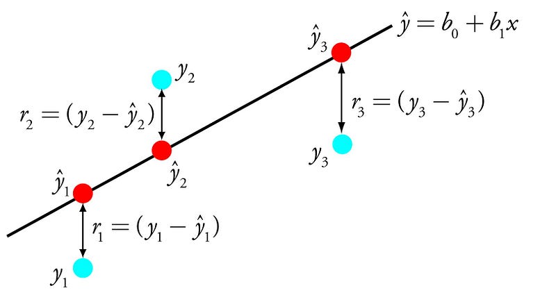
The portrayal of direct relapse is a condition that depicts a line that best fits the connection between the info factors (x) and the yield factors (y), by discovering particular weightings for the information factors called coefficients (B).
Straight Regression
For instance: y = B0 + B1 * x
We will anticipate y given the info x and the objective of the straight relapse machine learning online training calculation is to discover the qualities for the coefficients B0 and B1.
Diverse methods can be utilized to take in the direct relapse show from information, for example, a straight variable based math answer for standard minimum squares and slope plummet advancement.
Direct relapse has been around for over 200 years and has been broadly examined. Some great general guidelines when utilizing this method are to expel factors that are fundamentally the same as (connected) and to expel clamor from your information, if conceivable. It is a quick and basic procedure and great first calculation to attempt.
2 . Logistic Regression
Strategic relapse is another system obtained by machine gaining from the field of measurements. It is the go-to technique for twofold order (issues with two class esteems).
Strategic relapse resembles straight relapse in that the objective is to discover the qualities for the coefficients that weight each info variable. Not at all like straight relapse, the expectation for the yield is changed utilizing a non-direct capacity called the calculated capacity.
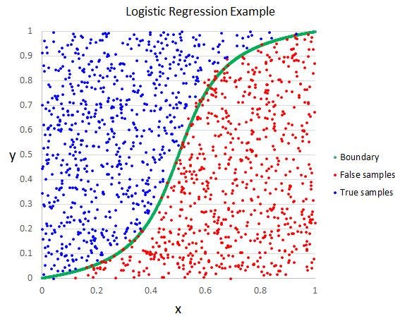
The calculated capacity resembles a major S and will change any an incentive into the range 0 to 1. This is helpful in light of the fact that we can apply a manage to the yield of the strategic capacity to snap esteems to 0 and 1 (e.g. On the off chance that under 0.5 at that point yield 1) and anticipate class esteem.
Calculated Regression
Due to how the model is found out, the expectations made by strategic relapse can likewise be utilized as the likelihood of a given information example having a place with class 0 or class 1. This can be valuable for issues where you have to give more justification for a forecast.
Like direct relapse, strategic relapse improves when you evacuate ascribes that are irrelevant to the yield variable and additional properties that are fundamentally the same as (corresponded) to each other. It's a quick model to learn and powerful on paired order issues.
3. Linear Discriminant Analysis
Calculated Regression is a grouping calculation customarily constrained to just two-class characterization issues. In the event that you have in excess of two classes then the Linear Discriminant Analysis calculation is the favored straight order system.
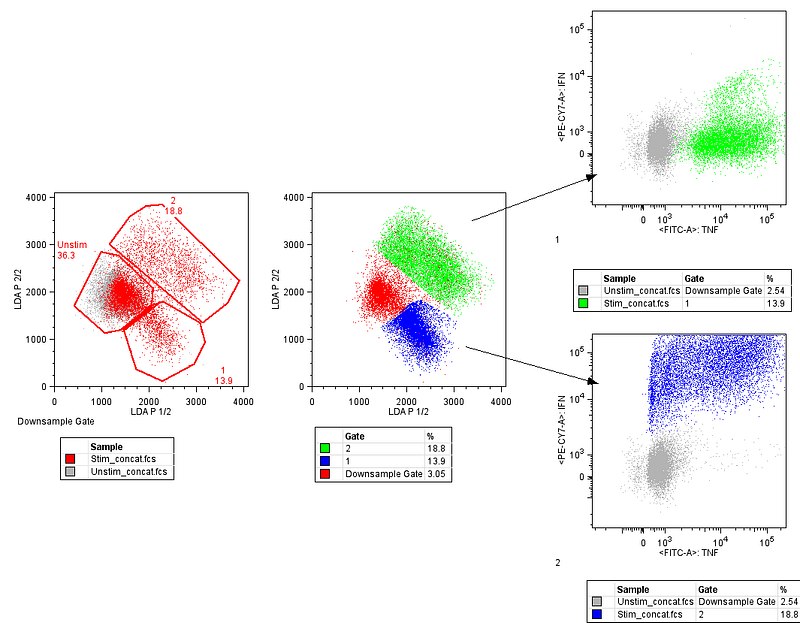
The portrayal of LDA is quite straightforward. It comprises factual properties of your information, computed for each class. For a solitary information variable this incorporates:
1. The mean an incentive for each class.
2. The change ascertained over all classes.
Direct Discriminant Analysis
Forecasts are made by ascertaining a separate an incentive for each class and making an expectation for the class with the biggest esteem. The strategy expects that the information has a Gaussian circulation (chime bend), so it is a smart thought to expel anomalies from your information beforehand. It's a straightforward and great technique for order prescient displaying issues.
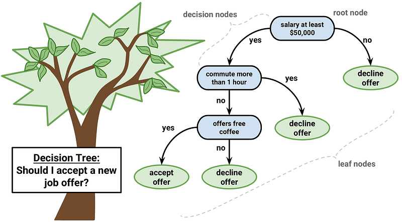
4. Classification and Regression Trees
The portrayal of the choice tree demonstrate is a double tree. This is your parallel tree from calculations and information structures, nothing excessively extravagant. Every hub speaks to a solitary information variable (x) and a split point on that factor (expecting the variable is numeric).
Choice Tree
The leaf hubs of the tree contain a yield variable (y) which is utilized to make an expectation. Expectations are made by strolling the parts of the tree until landing at a leaf hub and yield the class an incentive at that leaf hub.
Trees are quick to learn and quick to make expectations. They are additionally regularly exact for an expansive scope of issues and don't require any extraordinary planning for your information.
5. Naive Bayes
Credulous Bayes is a basic yet shockingly great calculation for prescient displaying.
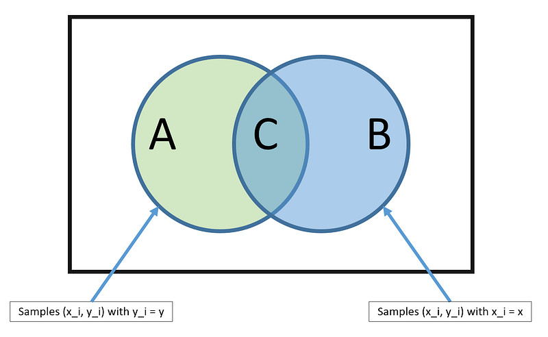
The model has included two kinds of probabilities that can be figured straightforwardly from your preparation information:
1) The likelihood of each class; and
2) The restrictive likelihood for each class given every x esteem.
Once ascertained, the likelihood model can be utilized to make forecasts for new information utilizing Bayes Theorem. At the point when your information is genuinely esteemed usually to accept a Gaussian circulation (ringer bend) with the goal that you can without much of a stretch gauge these probabilities.
Bayes Theorem
Credulous Bayes is called guileless in light of the fact that it accepts that each information variable is autonomous. This is a solid presumption and unlikely for genuine information, all things considered, the procedure is exceptionally viable on an extensive scope of complex issues.
6. K-Nearest Neighbors
The KNN calculation is extremely basic and exceptionally powerful. The model portrayal for KNN is the whole preparing dataset. Straightforward right?
Forecasts are made for another information point via seeking through the whole p ofreparing set for the K most comparative occurrences (the neighbors) and condensing the yield variable for those K examples. For relapse issues, this may be the mean yield variable, for characterization issues this may be the mode (or most normal) class esteem.
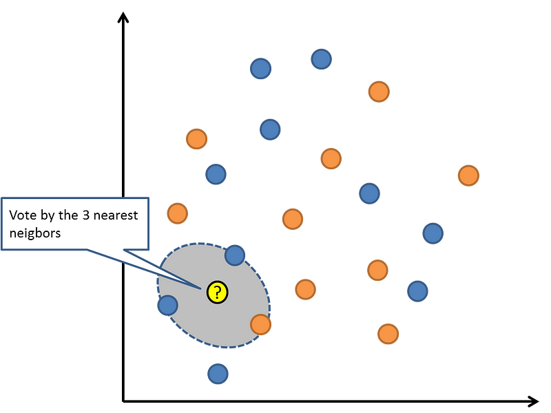
The trap is in how to decide the similitude between the information cases. The easiest method if your characteristics are the majority of a similar scale (all in crawls for instance) is to utilize the Euclidean separation, a number you can compute specifically in view of the contrasts between each information variable.
K-Nearest Neighbors
KNN can require a ton of memory or space to store the majority of the information, however just plays out an estimation (or realize) when an expectation is required, in the nick of time. You can likewise refresh and minister your preparation occasions after some time to keep forecasts exact.
Distance or closeness can separate in high measurements (heaps of info factors) which can contrarily influence the execution of the calculation on your concern. This is known as the scourge of dimensionality. It recommends you just utilize those information factors that are most pertinent to foreseeing the yield variable.
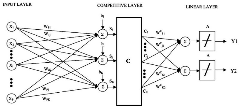
7. Learning Vector Quantization
A drawback of K-Nearest Neighbors is that you have to hold tight to your whole preparing dataset. The Learning Vector Quantization calculation (or LVQ for short) is a fake neural system calculation that enables you to pick what number of preparing occurrences to cling to and realizes precisely what those examples should resemble.
Learning Vector Quantization
The portrayal of LVQ is an accumulation of codebook vectors. These are chosen haphazardly first and foremost and adjusted to best outline the preparation dataset over various cycles of the learning calculation. After scholarly, the codebook vectors can be utilized to make forecasts simply like K-Nearest Neighbors. The most comparable neighbor (best coordinating codebook vector) is found by ascertaining the separation between each codebook vector and the new information case. The class esteem or (genuine incentive on account of relapse) for the best coordinating unit is then returned as the expectation. Best outcomes are accomplished in the event that you rescale your information to have a similar range, for example, somewhere in the range of 0 and 1.
On the off chance that you find that KNN gives great outcomes on your dataset take a stab at utilizing LVQ to lessen the memory prerequisites of putting away the whole preparing dataset.
8. Support Vector Machines
Bolster Vector Machines are maybe a standout amongst the most prominent and discussed online machine learning calculations.
A hyperplane is a line that parts the info variable space. In SVM, a hyperplane is chosen to best separate the focuses in the info variable space by their class, either class 0 or class 1. In two measurements, you can imagine this as a line and how about we accept that the majority of our info focuses can be totally isolated by this line. The SVM learning calculation finds the coefficients that outcomes in the best partition of the classes by the hyperplane.
Bolster Vector Machine
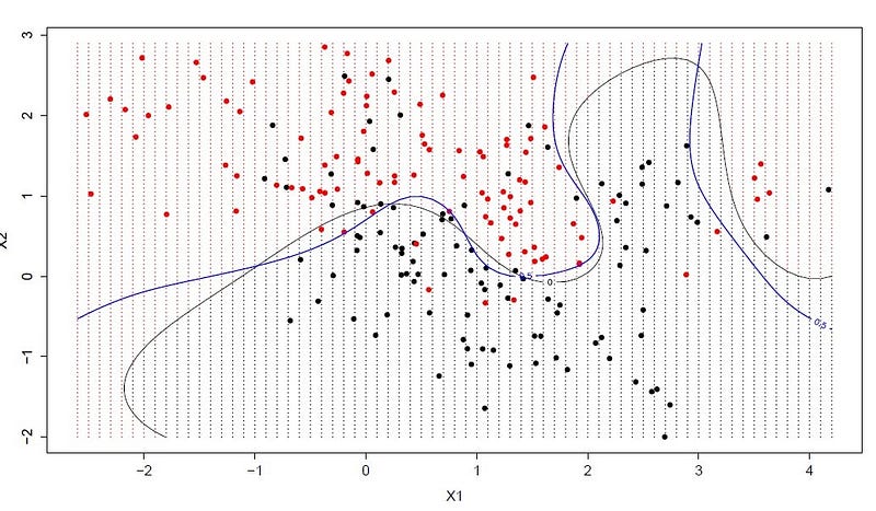
The separation between the hyperplane and the nearest information indicates is alluded as the edge. The best or ideal hyperplane that can isolate the two classes is the line that has the biggest edge. Just these focuses are important in characterizing the hyperplane and in the development of the classifier. These focuses are known as the help vectors. They bolster or characterize the hyperplane. By and by, an enhancement calculation is utilized to discover the qualities for the coefficients that augments the edge.
SVM may be a standout amongst the most great out-of-the-crate classifiers and worth attempting on your dataset.
9. Bagging and Random Forest
Arbitrary Forest is a standout amongst the most prominent and most intense machine learning calculations. It is a sort of troupe machine learning calculation called Bootstrap Aggregation or sacking.
The bootstrap is a great factual technique for evaluating an amount from an information test. For example, a mean. You take heaps of tests of your information, figure the mean, at that point normal the majority of your mean qualities to give you a superior estimation of the genuine mean esteem.
In packing, a similar approach is utilized, however rather to appraise whole measurable models, most regularly choice trees. Numerous examples of your preparation information are taken at that point models are developed for every datum test. When you have to make a forecast for new information, each model makes an expectation and the expectations are found the middle value of to give a superior gauge of the genuine yield esteem.
Irregular Forest
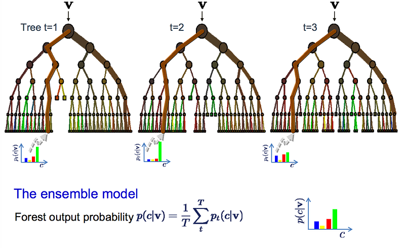
Irregular backwoods is a change on this approach where choice trees are made with the goal that instead of choosing ideal split focuses, imperfect parts are made by presenting haphazardness.
The models made for each example of the information are along these lines more not quite the same as they generally would be, yet at the same time exact in their one of a kind and diverse ways. Consolidating their expectations results in a superior gauge of the genuine fundamental yield esteem.
On the off chance that you get great outcomes with a calculation with high change (like choice trees), you can regularly improve results by sacking that calculation.
10. Boosting and AdaBoost
Boosting is a troupe system that endeavors to make a solid classifier from various frail classifiers. This is finished by building a model from the preparation information, at that point making a second model that endeavors to revise the mistakes from the main model. Models are included until the point when the preparation set is anticipated flawlessly or a most extreme number of models are included.
AdaBoost was the principal extremely effective boosting calculation created for twofold grouping. It is the best beginning stage for understanding boosting. Current boosting strategies expand on AdaBoost, most strikingly stochastic slope boosting machines.
AdaBoost
AdaBoost is utilized with short choice trees. After the principal tree is made, the execution of the tree on each preparation occasion is utilized to weight how much consideration the following tree that is made should focus on each preparation occurrence. Preparing information that is difficult to foresee is given more weight, though simple to anticipate occasions are given less weight. Models are made successively in a steady progression, each refreshing the weights on the preparation occurrences that influence the performed by the following tree in the arrangement. After every one of the trees are manufactured, expectations are made for new information, and the execution of each tree is weighted by how exact it was on preparing information.
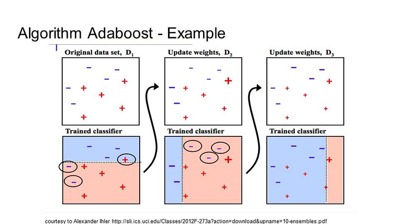
Since so much consideration is put on amending botches by the calculation it is vital that you have clean information with exceptions evacuated.


No comments:
Post a Comment